통계분석 결과 그래프

다음 그래프들은 전자책 파이썬과 함께하는 통계이야기 6 장과 7장에 수록된 그림들의 코드들입니다.

import numpy as np 
import pandas as pd
from scipy import stats
from sklearn.preprocessing import StandardScaler
import FinanceDataReader as fdr
import yfinance as yf
import statsmodels.api as sm
from statsmodels.formula.api import ols
from sklearn.linear_model import LinearRegression
import matplotlib.pyplot as plt
import seaborn as sns
sns.set_style("darkgrid")

#fig 611
st=pd.Timestamp(2024,1, 1)
et=pd.Timestamp(2024, 5, 30)
code=["^KS11", "^KQ11", "^DJI", "KRW=X"]
nme=['kos','kq','dj','WonDol']
da=pd.DataFrame()
for i in code:
    x=yf.download(i,st, et)['Close']
    x1=x.pct_change()
    da=pd.concat([da, x1], axis=1)
da.columns=nme
da1=da.dropna()
da1.index=range(len(da1))
da2=pd.melt(da1, value_vars=['kos', 'kq', 'dj', 'WonDol'], var_name="idx", value_name="val")
model=ols("val~C(idx)", data=da2).fit()
res=model.resid

plt.figure(figsize=(3,2))
varQQplot1=stats.probplot(res, plot=plt)
plt.show()

#fig 612, fig 611 데이터에서 이상치 제외한 모델의 잔차에 대한 QQ plot
from statsmodels.stats.outliers_influence import outlier_test
outl=outlier_test(model)
out2=np.where(outl.iloc[:,2]<1)[0]
da3=da2.drop(out2)
model1=ols("val~C(idx)", data=da3).fit()
res1=model1.resid

plt.figure(figsize=(3,2))
varQQplot1=stats.probplot(res1, plot=plt)
plt.show()

#fig 711
h=np.linspace(0, 5)
f=0.1*9.8*h
plt.figure(figsize=(4,3))
plt.plot(h, f, color="g", label="F=mgh\nm:0.1 kg")
plt.xlabel("h(m)")
plt.ylabel("F(N)")
plt.legend(loc="best")
plt.show()

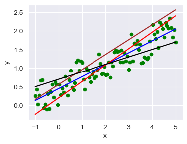
#fig 712
np.random.seed(3)
x=np.linspace(-1, 5, 100)
y=0.3*x+np.random.rand(100)
y1=0.56+0.4*x
y2=0.45+0.32*x
y3=0.2+0.44*x
y4=0.7+0.2*x
col=["brown",'b','r','k']
plt.figure(figsize=(4,3))
plt.scatter(x, y, color="g", s=20)
for i, j in enumerate([y1, y2, y3, y4]):
    plt.plot(x, j, color=col[i])
plt.xlabel("x")
plt.ylabel("y")
plt.show()

#fig 721
st=pd.Timestamp(2021,1, 1)
et=pd.Timestamp(2024, 5, 10)
kos=fdr.DataReader('KS11',st, et)[["Open","Close"]]
kos.index=range(len(kos))
X=kos.values[:,0].reshape(-1,1)
y=kos.values[:,1].reshape(-1,1)
#독립변수 정규화(표준화)
xScaler=StandardScaler().fit(X)
X_n=xScaler.transform(X)
#반응변수 정규화(표준화)
yScaler=StandardScaler().fit(y)
y_n=yScaler.transform(y)

plt.figure(figsize=(4,2))
plt.scatter(X_n, y_n, label="Data")
plt.plot(X_n, 0.998*X_n, color="red", label="Regression line")
plt.legend(loc="best", frameon=False)
plt.xlabel("Open", weight="bold")
plt.ylabel('Close', weight="bold")
plt.show() 

#fig 731
x=np.linspace(-2, 2, 100)
y=x**2
x1=np.linspace(-2, 0, 50)
y1=-2*x1-1
x2=np.linspace(0, 2, 50)
y2=2*x2-1
plt.figure(figsize=(4,3))
plt.plot(x, y, color="g", label=r"SSE=$(y_i-bx_i)^2$")
plt.plot(x1, y1, color="brown", ls="--", label=r"$\frac{d\;SSE}{dx}>0$" )
plt.plot(x2, y2, color="b",  ls="--", label=r"$\frac{d\;SSE}{dx}<0$" )
plt.hlines(0, -2, 2, ls="--", color="k", label=r"$\frac{d\;SSE}{dx}=0$")
plt.xlabel("x")
plt.ylabel("SSE")
plt.legend(loc="best",prop={'size':10}, labelcolor='linecolor', frameon=False)
plt.show()

#fig 751
x=np.linspace(-1, 2, 100)
y=x+0.5
plt.figure(figsize=(4,3))
plt.plot(x, y, color="g", label="regression")
plt.hlines(1.7, -1, 2, color="k", ls="--", label="mean line")
plt.scatter(0.25, 1.7, s=20, color="k", label=r"$\bar{y}$")
plt.scatter(0.25, 0.75, s=20, color="r", label=r"$\hat{y}$")
plt.scatter(0.25, 0, s=20, color="b", label=r"$y_{obs}$")
plt.vlines(0.25, 0.75, 1.7, color="r", ls="--")
plt.vlines(0.25, 0, 0.75, color="b", ls="--")
plt.vlines(0.18, 0, 1.7, color="k", ls="--", alpha=0.7)
plt.text(0.3, 1.2, r"SSReg=$(\bar{y}-\hat{y})^2$", color="r", weight="bold", size=8)
plt.text(0.3, 0.25, r"SSE=$(y_{obs}-\hat{y})^2$", color="b", weight="bold", size=8)
plt.text(-0.9, 0.7, r"SST=$(y_{obs}-\bar{y})^2$", color="k", weight="bold", size=8)
plt.xlabel("x")
plt.ylabel("y")
plt.xlim(-1.1, 2.5)
plt.legend(loc="lower right", prop={'size':8}, frameon=False)
plt.show()

#fig 752 ~ fig 758에 사용되는 데이터
st=pd.Timestamp(2021,1, 1)
et=pd.Timestamp(2024, 5, 10)
kos=fdr.DataReader('KS11',st, et)[["Open","Close"]]
kos.index=range(len(kos))
X=kos.values[:,0].reshape(-1,1)
y=kos.values[:,1].reshape(-1,1)
#독립변수 정규화(표준화)
xScaler=StandardScaler().fit(X)
X_n=xScaler.transform(X)
#반응변수 정규화(표준화)
yScaler=StandardScaler().fit(y)
y_n=yScaler.transform(y)

#fig 752
mod = LinearRegression()
mod.fit(X_n, y_n)
pre=mod.predict(X_n)
err=pre-y_n
plt.figure(figsize=(3,2))
errorRe=stats.probplot(err.ravel(), plot=plt)
plt.show()

#fig753
X_n0=sm.add_constant(X_n)
reg=sm.OLS(y_n, X_n0).fit()
influence=reg.get_influence()
infSummary=influence.summary_frame()
hat=infSummary["hat_diag"]
plt.figure(figsize=(6, 2))
plt.stem(hat)
plt.axhline(np.mean(hat), c='g', ls="--", label=r"$\mu_{lv}$")
plt.axhline(np.mean(hat)*2, c='brown', ls="--", label=r"$2\mu_{lv}$")
plt.xlabel('Data index')
plt.ylabel("Leverage (lv)")
plt.legend(loc="best", labelcolor="linecolor")
plt.title("leverage")
plt.show()

#fig754
out1id=np.where(hat>2*hat.mean())[0]
X_n0Hat=np.delete(X_n0, out1id, axis=0)
y_nHat=np.delete(y_n, out1id, axis=0)
reg_hat=sm.OLS(y_nHat, X_n0Hat).fit()
plt.figure(figsize=(6, 2))
plt.subplots_adjust(wspace=0.5)
plt.subplot(1,2,1)
stats.probplot(reg.resid, plot=plt)
plt.title("a) Probability plot")
plt.subplot(1,2,2)
stats.probplot(reg_hat.resid, plot=plt)
plt.title("b) Probability plot")
plt.show()

res_std=infSummary["student_resid"]
plt.figure(figsize=(6, 3))
plt.subplots_adjust(hspace=0.6)
plt.subplot(2,1,1)
plt.stem(reg.resid)
plt.ylabel("Resid.")
plt.title("a) Residual")
plt.subplot(2,1,2)
plt.stem(res_std)
plt.axhline(3, c='g', ls='--')
plt.axhline(-3, c='g', ls='--')
plt.xlabel("Data index")
plt.ylabel("Student Resid.")
plt.yticks([-3, 0, 3])
plt.title("b) Studenized Residual")
plt.show()

#fig 756
out_stres=np.where(np.abs(res_std)>3)[0]
ind_stres=np.delete(X_n0, out_stres, axis=0)
de_stres=np.delete(y_n, out_stres, axis=0)
reg_stres=sm.OLS(de_stres, ind_stres).fit()
plt.figure(figsize=(3,2))
fig=stats.probplot(reg_stres.resid, plot=plt)
plt.show()

#fig757
cook=infSummary["cooks_d"]
cd_ref=4/(len(reg.resid)-2-1)
cd_idx=np.where(cook>cd_ref)[0]
ind_cd=np.delete(X_n0, cd_idx, axis=0)
de_cd=np.delete(y_n, cd_idx, axis=0)
reg_cd=sm.OLS(de_cd, ind_cd).fit()

plt.figure(figsize=(3,2))
fig=stats.probplot(reg_cd.resid, plot=plt)
plt.show()

#fig758
dffi=infSummary["dffits"]
dff_ref=2*np.sqrt(3/(len(reg.resid)-2+1))
dff_idx=np.where(dffi>dff_ref)[0]
ind_dff=np.delete(X_n0, dff_idx, axis=0)
de_dff=np.delete(y_n, dff_idx, axis=0)
reg_dff=sm.OLS(de_dff, ind_dff).fit()
plt.figure(figsize=(3,2))
fig=stats.probplot(reg_dff.resid, plot=plt)
plt.show()

#fig 761 ~ fig 763에 사용된 데이터 
st=pd.Timestamp(2023,1, 10)
et=pd.Timestamp(2024, 5, 30)
code=["^KS11", "^KQ11", "122630.KS", "114800.KS","KRW=X","005930.KS"]
nme=["kos","kq","kl", "ki", "WonDol","sam" ]
da=pd.DataFrame()
for i, j in zip(nme,code):
    x=yf.download(j,st, et)["Close"]
    da=pd.concat([da, x], axis=1 )
da.columns=nme
da.index=pd.DatetimeIndex(da.index.date)
da2=da.ffill()
ind=da2.values[:-1,:-1]
de=da2.values[1:,-1].reshape(-1,1)
final=da2.values[-1, :-1].reshape(1,-1)
indScaler=StandardScaler().fit(ind)
deScaler=StandardScaler().fit(de)
indNor=indScaler.transform(ind)
finalNor=indScaler.transform(final)
deNor=deScaler.transform(de)
da3=pd.DataFrame(np.c_[indNor, deNor.reshape(-1,1)])
da3.columns=da2.columns
form='sam~kos+kq+kl+ki+WonDol'
reg=ols(form, data=da3).fit()
re=reg.summary()
mod=LinearRegression().fit(indNor, deNor)

#fig 761
plt.figure(figsize=(4, 3))
plt.plot(deNor, c="g", ls="--", label="data")
plt.plot(mod.predict(indNor), c="b", label="regression")
plt.xlabel("Data index")
plt.ylabel("Standardized response variables")
plt.legend(loc="best", frameon=False)
plt.show()

#fig762
err=reg.resid
plt.figure(figsize=(4,3))
stats.probplot(err, plot=plt, rvalue=True)
plt.show()

#fig763
fig=plt.figure(figsize=(4, 3))
plt.stem(reg.resid_pearson)
plt.axhline(3, c="g", ls="--")
plt.axhline(-3, c="g", ls="--")
plt.xlabel("Data index")
plt.ylabel("Student Resid.")
plt.yticks([-3, 0, 3, 6])
plt.title("student Resid.")
plt.show()