Contents

1. Probability and Expected Value
   1. Expected value
   2. Linear combination of expected values

Probability and Expected Value

A quantitative indicator for mathematically describing the characteristics and shape of random variables and probability distributions is called moment.

$$\begin{aligned}&\text{nth order moment }= E(x^n)\\ &n= 1, 2, \cdots \end{aligned}$$

Moments are used to derive various statistics such as skewness and kurtosis along with mean and variance introduced in descriptive statistics.

Expected value

The mean is the most commonly used statistic to characterize variables. This statistic is calculated as the product of the frequency and probability for each variable value and is called expected value(E(X)).

Each value of the random variable X can be specified by the relative likelihood, that is, the probability function, which is the probability that the value can appear compared to other values. When the variable is discrete, it is called probability mass function , and when the variable is continuous, it is classified as probability density function. It is also called the probability density function without distinction. The probability density function is expressed as f(x), and the cumulative probability function, which is the sum (integral) of the functions, is expressed as F(x). Using this probability density function, the mean, which is the first moment, can be formulated as Equation 1.

$$\begin{equation} \begin{aligned}&\mu=E(X)=\sum^n_{i=0} x_iP(X=x_i), \qquad P(X):\text{probability of occurrence }\\ &\qquad \Updownarrow \\ &E(X^n)=\begin{cases}\sum_{x \in \mathbb{R}}x^n f(x)& \text{discrete variable}\\ \int^\infty_{-\infty}x^n f(x)\, dx& \text{continuous variable} \end{cases}\\ &\mathbb{R}: \text{Real number}\\ &n:0, 1, 2, \cdots \end{aligned} \end{equation}$$

Example 1)
  Let's calculate the average score if Student A's 4 scores in a statistics course during a semester were 82, 75, 83, and 90 respectively.

$$\text{mean}=\frac{82+75+83+90}{4}=82.5$$

import numpy as np
import pandas as pd
import matplotlib.pyplot as plt
from sympy import *

data=np.array([82, 75, 83, 90])
pmf=1/4
data.mean()

82.5

The probability that one of the four values above will be selected is $\displaystyle \frac{1}{4}$. This probability is for a discrete random variable and becomes a function of the probability mass. Taking this function into account, the mean can be calculated as

$$\text{mean}=82\cdot \frac{1}{4}+75\cdot \frac{1}{4}+83\cdot \frac{1}{4}+90\cdot \frac{1}{4}=82.5$$

np.sum(data*pmf)

82.5

However, if different weights are applied to each test, the weight becomes the probability that 4 values will be selected.

weight=np.array([1/10, 2/10, 3/10, 4/10])
dataWeig=weight*data
dataWeig

array([ 8.2, 15. , 24.9, 36. ])

dataWeig.sum()

84.1

Example 2)
If the number of points occurring in one dice trial is a random variable, try to determine the distribution of the values of that variable.

x=np.array([i for i in range(1, 7)])
x

array([1, 2, 3, 4, 5, 6])

The probability of each value is uniform as $\displaystyle \frac{1}{6}$. A graph of this uniform probability is shown in Figure 1. This distribution is called uniform distribution.

plt.figure(figsize=(5, 3))
plt.scatter(x, np.repeat(1/6, 6), label=r'p(x)=$\frac{1}{6}$')
plt.xlabel('x', size="13", weight='bold')
plt.ylabel('PMF', size="13", weight='bold')
plt.legend(loc='best',prop={'size':13})
plt.text(0, 0.152, "Figure 1. Probability mass function in one dice trial.", size=13, weight="bold")
plt.show()

The expected values for this trial are:

E=np.sum(x*Rational('1/6'))
E

$\displaystyle \frac{7}{2}$

The expected value, which is the first moment for a new variable transformed by the random variable X, is linearly combined as shown in Equation 2.

$$\begin{equation}\tag{2} \begin{aligned} E(aX+b)&=aE(x)+b \\ &\qquad \Downarrow\\ E(aX+b)&=\int^\infty_{-\infty}(ax+b)f(x)\,dx\\ &=\int^\infty_{-\infty}ax \cdot f(x)\,dx+\int^\infty_{-\infty}b \cdot f(x)\, dx\\ &=a\int^\infty_{-\infty}x \cdot f(x)\,dx+b\int^\infty_{-\infty}f(x)\,dx\\ &=a\int^\infty_{-\infty}x \cdot f(x)\,dx+b\\ &=aE(x)+b\\ \because \;& \text{sum of all probabilities }: \; \int^\infty_{-\infty}f(x)\,dx=1\end{aligned}\end{equation}$$

Example 3)
  What is the expected value if the random variable X is the number of heads in the trial of tossing 3 coins?
This problem can be approached in the following way.:

• Determine the sample space S of the events that can occur in the trial
• The random variable becomes 0, 1, 2, 3 as the number of occurrences of heads, and the frequency of occurrence of each event in S is calculated (using the np.unique() function)
• $\displaystyle \text{probability mass function}=\frac{\text{frequency of each event}}{\text{total number of S}}$
• Calculate expected value

#head:1, tail:0
x=np.array([0,1,2,3])
E=[0,1]
S=np.array([(i,j, k) for i in E for j in E for k in E ])
S

array([[0, 0, 0],
        [0, 0, 1],
        [0, 1, 0],
        [0, 1, 1],
        [1, 0, 0],
        [1, 0, 1],
        [1, 1, 0],
        [1, 1, 1]])

S1=np.sum(S, axis=1)
S1

array([0, 1, 1, 2, 1, 2, 2, 3])

val, fre=np.unique(S1, return_counts=True)
val

array([0, 1, 2, 3])

fre

array([1, 3, 3, 1])

pInd=fre/len(S1)
pInd

array([0.125, 0.375, 0.375, 0.125])

Ex=np.sum(val*pInd)
Ex

1.5

Example 4)
  What is the expected value of a random continuous variable with the following probability density function (pdf)?

$$f(x)=\begin{cases}c(x^3+x^2+1), &0In the above function, the integral over the range (0, 10) should be 1. By applying this condition, the constant c can be calculated.

The integral calculation applies the function integrate() from the Python library sympy. Also, the unknown (c) expressed in the result of the integration can be determined using the sympy function solve().

c, x=symbols("c x")
f=c*(x**3+x**2+1)
F=f.integrate((x, 0, 10))
F

$\displaystyle \frac{8530 c}{3}$

C=solve(Eq(F,1), c)
C

[3/8530]

By substituting C in the above result, the probability density function is written as follows.

f1=f.subs(c, C[0])
f1

$\displaystyle \frac{3 x^{3}}{8530} + \frac{3 x^{2}}{8530} + \frac{3}{8530}$

The expected value for the determined probability density function is:

E=integrate(x*f1, (x, 0, 10))
E

$\displaystyle \frac{6765}{853}$

If the random variable is the result of another function, that is, the expected value of the random variable Y(Y=g(X)) based on the random variable X and applying another function can be defined as Equation 3.

$$\begin{align}\tag{3} &E(g(x))=\begin{cases} \sum_{x \in R} g(x)f(x),& \quad \text{discrete variable } \\ \int^\infty_{-\infty} g(x)f(x)\, dx, & \quad \text{continuous variable} \end{cases}\\ &R: \forall x \end{align}$$

Example 5)
  If the number of odd numbers is X when the die is rolled 4 times, then E(X) and E(X²)?

In this trial, if the random variable X that considers odd (1, 3, 5) to be 1 and even (2, 4, 6) to be 0, this trial is repeated 4 times. The range of X values is as follows:

S={0, 1, 2 , 3, 4}

This trial can be computed using the scipy.special.comb() function for calculating combinations. Also, since it is a binomial variable having two variables, odd (0) and even (1), the probability mass function of the binomial distribution can be calculated using the scipy.stats.pmf() function.

from scipy import special
special.comb(4, 0)*(1/2)**0*(1/2)**4

0.0625

from scipy import stats
stats.binom.pmf(0, 4, 1/2)

0.0625

In the above way, the probability and expected value for each value of S can be calculated. In addition, several methods of scipy.stats.binom() that can calculate various statistics of the binomial distribution can be applied to produce results without intermediate calculations.

S=np.array([0,1,2,3, 4])
p=np.array([special.comb(4, i)*(1/2)**i*(1/2)**(4-i) for i in S])
p

array([0.0625, 0.25 , 0.375 , 0.25 , 0.0625])

EX1=np.sum(S*p)
EX1

2.0

p=stats.binom.pmf(S, 4, 1/2)
p

array([0.0625, 0.25 , 0.375 , 0.25 , 0.0625])

np.sum(S*p)

2.0000000000000004

stats.binom.expect(args=(4, 1/2))

2.0000000000000004

In this example, the random variable is a trial of taking one from 0, 1, 2, 3, 4. As shown in Figure 2, if the expected value (average) is simulated when the same test is repeated, the probability of the same value as the above result is highest.

Example 6)
  In the example above, if $X^2$ is used instead of X for the random variable, E(X²)?

EX2=np.sum(S**2*p)
EX2

5.000000000000001

Example 7)
  The following is the PDF definition of a continuous random variable.

$$f(x)=\begin{cases} 1& \quad 0Based on the continuous random variable X, determine the expected value of a new random variable Y=g(X)=e^x and the expected value of e^x3.

$$\begin{aligned}E(e^x)&=\int^1_0 e^xf(x)\,dx\\ &=\int^1_0 e^x\,dx \\ E(e^{x^3})&=\int^1_0 e^{x^3}f(x)\,dx\\ &=\int^1_0 e^{x^3}\,dx \end{aligned}$$

Calculations can be applied to sympy's integrate() function, and the result can be an expression consisting of symbols or numbers. These results can be converted to numbers using N().

x=symbols('x')
re1=integrate(exp(x), (x, 0, 1))
re1

$\displaystyle -1 + e$

N(re1, 3)

$\displaystyle 1.72$

re3=integrate(exp(x**3), (x, 0, 1))
N(re3, 3)

$\displaystyle 1.34$

Example 8)
  It is said that two books are used in one statistics lecture. It is assumed that the purchase of the two books is independent. In other words, it is assumed that the purchase of the main material does not affect the purchase of the auxiliary material. Under that assumption, the probability of purchasing or not purchasing a book per student is the same, so it can be considered as a random variable. In this case, the random variable consists of when students buy both books, when they buy only the main textbook, when they buy only the auxiliary textbook, and when they don't buy both books. The following shows the tendency of students to purchase books in the past.

case	probiity
no both books	10%
main book	45%
sub-book	25%
both books	20%

Using the probabilities of each case from the existing data presented above, and assuming that the prices of the main textbook and sub-textbook are \$ 100 and \$ 70, respectively, it can be summarized as follows.

case	1	2	3	4	total
x(price)	0	100	70	170	340
P(X=x)(probability)	0.1	0.45	0.25	0.2	1

Calculate the average book purchase cost per student for this course:

da=pd.DataFrame([[0,100,70,170],[0.1,0.45,0.25,0.2]],
                index=["price","probability"], columns=[1,2,3,4])
da

	1	2	3	4
price	0.0	100.00	70.00	170.0
probability	0.1	0.45	0.25	0.2

Ex1=da.product(axis=0)
Ex1

1     0.0
    2    45.0
    3    17.5
    4    34.0
    dtype: float64

Ex=Ex1.sum()
Ex

96.5

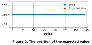
Graphing the above data to find the location of the expected value is as follows.

plt.figure(figsize=(6, 2))
plt.plot(da.iloc[0,:], np.repeat(0.5, 4), 'o-', label="price")
plt.scatter(Ex, 0.5, color="red", label="Expected Vlue")
plt.xlabel("Price", size="13", weight="bold")
plt.legend(loc="best")
ax=plt.gca()
#ax.axes.yaxis.set_visible(False)
plt.grid()
plt.text(0, 0.44, "Figure 2. The position of the expected value.", size=13, weight="bold")
plt.show()

Linear combination of expected values

It is often necessary to consider the expected value in the combination of multiple independent events. For example, someone (A) goes to work five days a week. Consider the following to create a probability distribution for the amount of time (W) taken to work per week:

• The total work hours for a week is the result of adding up all work hours from Monday to Friday (W)
• Each attendance time is a random variable with the same probability.
• Each attendance time is independent because it does not affect each other.
• The start time for each day of the week is X₁, …, X₅

W=X₁+X₂+X₃+X₄+X₅

If the average daily commute time is 30 minutes, it can be expressed as follows.

$$\begin{aligned} E(W)&=E(X_1+X_2+X_3+X_4+X_5)\\&=E(X_1)+E(X_2)+E(X_3)+E(X_4)+E(X_5) \end{aligned}$$

Consequently, the expected value of the total time is equal to the sum of the expected values of the individual time. This can be generalized as Equation 4.

The expected value of the sum of random variables is equal to the sum of the expected values of the individual random variables.

$$\begin{equation}\tag{4} E(X_1+X_2+\cdots+X_k) = E(X_1) + E(X_2) + \cdots + E(X_k) \end{equation}$$

Equation 4 is called **linear combination** of random variables. For example, the expected value of a random variable Z generated by the sum of two random variables X and Y is calculated as follows.

$$\begin{aligned}&Z= aX + bY\\ & \text{a, b: constant} \\&\begin{aligned}E(Z)&=E(aX+bY)\\& =aE(X) + bE(Y)\end{aligned} \end{aligned}$$

Example 9)
 It bought 300 and 150 shares of Apple (ap) and Google (go), respectively. Calculate the expected return for two stocks over the next month based on the average daily rate of change between each stock's opening and closing prices.

The following data is daily stock price data for a certain period using the module function ``fdr.DataReader()`` of python library FinanceDataReader.

import FinanceDataReader as fdr
st=pd.Timestamp(2020,3, 1)
et=pd.Timestamp(2021, 11, 30)
ap=fdr.DataReader('AAPL', st, et)[['Open','Close']]
go=fdr.DataReader('GOOGL', st, et)[['Open','Close']]
data=pd.concat([ap, go], axis=1)
data.columns=[i+j for i in ["ap", "go"] for j in ["Open","Close"]]
data

	apOpen	apClose	goOpen	goClose
Date
2020-03-02	70.57	74.70	1351.4	1386.3
2020-03-03	75.92	72.33	1397.7	1337.7
2020-03-04	74.11	75.68	1359.0	1381.6
2020-03-05	73.88	73.23	1345.6	1314.8
2020-03-06	70.50	72.26	1269.9	1295.7
...	...	...	...	...
2021-11-23	161.12	161.41	2923.1	2915.6
2021-11-24	160.75	161.94	2909.5	2922.4
2021-11-26	159.57	156.81	2887.0	2843.7
2021-11-29	159.37	160.24	2880.0	2910.6
2021-11-30	159.99	165.30	2900.2	2837.9

443 rows × 4 columns

Calculating the expected values for ap and go requires calculating the values and probabilities of a particular interval. Therefore, it is necessary to convert the continuous variable, which is the rate of change between "Open" and "Close" of each stock, into a nominal variable. A nominal variable will be designed to have two classes, increase and decrease. To make a continuous variable into a nominal variable, use the pd.cut() function.

apChg=(data['apClose']-data['apOpen'])/data['apOpen']
apCat=pd.cut(apChg, bins=[-10, 0, 10], labels=[0, 1])
apCat.head(3)

Date
2020-03-02    1
2020-03-03    0
2020-03-04    1
dtype: category
Categories (2, int64): [0 < 1]

goChg=(data['goClose']-data['goOpen'])/data['goOpen']
goCat=pd.cut(goChg, bins=[-10, 0, 10], labels=[0, 1])
goCat.head(3)

Date
2020-03-02    1
2020-03-03    0
2020-03-04    1
dtype: category
Categories (2, int64): [0 < 1]

Create a crosstab for the above results.

crostab=pd.crosstab(apCat, goCat, rownames=['ap'], colnames=['go'], margins=True, normalize=True)
np.around(crostab,3)

go	0	1	All
ap
0	0.325	0.147	0.472
1	0.135	0.393	0.528
All	0.460	0.540	1.000

The difference between "Close" and "Open" in the raw data is the reward for this transaction. Therefore, the expected value is calculated as

Expected Value= difference mean in case of rise ‧increse probability + difference mean in case of decrese‧ decrese probability

Use the ``.groupby()`` method to calculate the average for each class of increase and decrease in a list variable. In order to apply this method, values that can be distinguished by class must be included in the object. Therefore, the difference between "Close" and "Open" and the categorical variable are combined using the ``pd.concat()`` function.

ap1=pd.concat([data['apClose']-data['apOpen'], apCat], axis=1)
ap1.columns=['diff','Cat']
ap1.head(3)

	diff	Cat
Date
2020-03-02	4.13	1
2020-03-03	-3.59	0
2020-03-04	1.57	1

go1=pd.concat([data['goClose']-data['goOpen'], goCat], axis=1)
go1.columns=['diff','Cat']
go1.head(3)

	diff	Cat
Date
2020-03-02	34.9	1
2020-03-03	-60.0	0
2020-03-04	22.6	1

Calculate the average for each class in the event and multiply the probability from the crosstab to calculate the expected value.

apMean=ap1.groupby(['Cat']).mean()
apMean

	diff
Cat
0	-1.434402
1	1.431239

apExp=np.dot(crostab.iloc[:-1,-1].values.reshape(1,-1), apMean.values)
apExp

array([[0.07927765]])

goMean=go1.groupby(['Cat']).mean()
goMean

	diff
Cat
0	-20.229412
1	19.602092

goExp=np.dot(crostab.iloc[-1, :-1].values.reshape(1,-1), goMean.values)
goExp

array([[1.25981941]])

If the object of the mean and probability calculated in the code above is converted to numpy type, it is a matrix and a vector as follows.

apMean.shape, crostab.iloc[:-1,-1].values.shape

((2, 1), (2,))

In the code above, the expected value is the matrix multiplication by converting the probability and mean into (1,2) and (2,1) using the .reshape() method.

The above result is the same as the result of calculating the average of the continuous variable itself, regardless of the class of increse and decrese.

apTotalMean=ap1['diff'].mean()
apTotalMean

0.07927765237020294

goTotalMean=go1['diff'].mean()
goTotalMean

1.2598194130925569

Expected values for the above two stocks are as follows:

E[aA+bB]=aE[A]+bE[b]     a, b: constant

TotalExp=300*apExp+150*goExp
print(TotalExp)

[[212.75620767]]

In the case of stocks, the above results may not reflect future estimates due to the variability of circumstances. However, if a situation similar to the calculation period occurs repeatedly, it may serve as a reference for trading. Because expected value means a value to maintain a balance between probabilistic and unexpected changes, examining the trend of expected value over various periods will help to understand information about stocks' fluctuations.

Example 10)
 The range of the random variable X is R_x={-3,-2,-1, 0, 1, 2, 3} and the probability mass function (f(x)) is $\displaystyle \frac{1}{7}$, determine the range and PMF of a new random variable Y=2|X+1| based on this variable.

The value of variable X is converted by function Y follow as:

RX=np.array([-3,-2,-1, 0, 1, 2, 3])
Y=2*abs(RX+1)
Y

array([4, 2, 0, 2, 4, 6, 8])

The probability of each value of variable Y is

val,fre=np.unique(Y, return_counts=True)
val

array([0, 2, 4, 6, 8])

fre

array([1, 2, 2, 1, 1])

P=[Rational(i, 7) for i in fre]
P

[1/7, 2/7, 2/7, 1/7, 1/7]

pd.DataFrame([val, P], index=['Y', 'P']).T

	Y	P
0	0	1/7
1	2	2/7
2	4	2/7
3	6	1/7
4	8	1/7

The above result shows that the probability mass function of y for each x is the same. However, the probability mass function is also transformed because it considers the frequencies for the variable Y. For example, the X variables -3 and 1 are both converted to 2 by the function Y. Therefore, the probability mass function is

$$\begin{aligned}f(Y=2)&=f(X=-3)+f(X+1)\\&=\frac{1}{7}+\frac{1}{7}\\&=\frac{2}{7} \end{aligned}$$

The above expression can be generalized as Equation 5.

\begin{equation}\tag{5} \begin{aligned}f(y)&=P(Y=y)\\&=P(g(x)=y)\\&=\sum_{x=g^{-1}(y)} f(x)\end{aligned} \end{equation}

The expected values for this example are:

EY=np.sum(val*fre)
Rational(EY, 7)

$\displaystyle \frac{26}{7}$