Inferential Statistics: Standard Deviation and Standard Error

Contents

1. Sampling distribution
2. Standard Deviation and Standard Error

Inferential Statistics

Statistical inference is an analytical method that estimates the parameters of a whole (population) with a part (sample). In general, it is often difficult or impossible to survey the population due to the constraints of several conditions. In this case, since the population parameters are unknown, they have to be estimated from sample. For example, it is difficult to obtain data on all stock prices that are traded. Therefore, various analyzes can be carried out under the assumption that statistics such as mean and variance of a sample that can be generated from the population or have characteristics similar to that population will be similar to the parameters. In this case, it is necessary to judge the rationality of the hypothesis that the statistic of the sample is similar to the parameter, and the basis for this judgment can be determined by statistical inference.

For example, in a study measuring the average height of 6th graders, the subject would be all 6th graders in the country. However, limited research time and cost can make the investigation of all subjects difficult. In this case, since population statistics cannot be calculated, the population mean can be substituted with the average of the results measured by randomly selecting a small group for each region. As shown in Table 1, for this study, all subjects would be population and selected portions would be sample.

Population and sample

Population	All subjects of study
Sample	The part that is actually measured or observed for research

Figure 1. Relationship between population and sample.

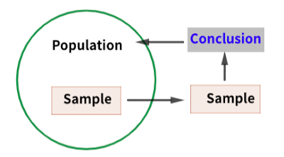
As shown in Figure 1, the conclusions from the sample apply to the population, so the sample must have representative. That is, the characteristics of the population must be reflected in the sample. However, although the sample is chosen from the population, the characteristics of the two populations cannot be completely matched. In other words, inherent differences exist and it is very important to recognize them. To indicate these differences, the signs of the statistic produced by each are distinguished. For example, the mean and standard deviation of the population are denoted by μ and σ, and the sample by $\bar{x}$ and s, respectively.

In order to draw statistical conclusions, the population and sample may be the same or strictly distinct, depending on the different conditions of the study. In the case of descriptive statistics introduced in Chapter 1, the population and sample are the same. Conversely, when a population and a sample are distinguished, a conclusion must be drawn for a larger population based on small information in the sample. This is called inference and this kind of statistic is called inference statistics. Inference statistics consist of estimation steps and hypothesis testing steps. Estimation is the step of estimating parameters, such as confidence intervals, and hypothesis testing is the step of testing whether the estimated value is reasonable.

Sampling distribution

In the ideal case of generating one sample from the population as follows, the population mean is equal to the mean of the sample means. That is, for two samples with three elements from a population with six elements, the following relationship holds:

$$\begin{align}&X={x_1, x_2, x_3, x_4, x_5, x_6}\\ &X_1={x_1, x_2, x_3}\\&X_2={x_4, x_5, x_6}\end{align}$$ $$\begin{align}& \mu=\frac{x_1+x_2+x_3+x_4+x_5+x_6}{6}\\&\bar{X_1}=\frac{x_1+x_2+x_3}{3}\\&\bar{X_2}=\frac{x_4+x_5+x_6}{3}\\\bar{X}&=\frac{\bar{X_1}+\bar{X_2}}{2}\\&=\frac{\frac{x_1+x_2+x_3}{3}+\frac{x_4+x_5+x_6}{3}}{2}\\&=\frac{x_1+x_2+x_3+x_4+x_5+x_6}{6}\\&=\mu \end{align}$$

Above, $\bar{X}_1$ and $\bar{x}_2$ may not be equal. As such, deviations exist between the sample means randomly sampled from the population. That is, the means form a distribution, and this distribution is called the sample mean distribution or sampling distribution. In inferential statistics, the mean of these sampling distributions, that is, sample mean, is used as the population mean. This estimate is called unbiased estimate. This means that the deviation between the population mean and the sample mean can be regarded as the noise level that occurs under normal circumstances, and consequently, it is assumed that the deviation will not have a major impact on the conclusion of the analysis. The basis for this assumption is based on the analysis of the sampling distribution.

Example 1)
The following data are the Dow Jones Indices over a period of time.

import numpy as np
import pandas as pd
import matplotlib.pyplot as plt
from scipy import stats

import FinanceDataReader as fdr
st=pd.Timestamp(2021,4, 1)
et=pd.Timestamp(2021, 12, 15)
da=fdr.DataReader("DJI", st, et)
da.head(2)

	Close	Open	High	Low	Volume	Change
Date
2021-04-01	33153.21	33054.58	33167.17	32985.35	318340000.0	0.0052
2021-04-05	33527.19	33222.38	33617.95	33222.38	345150000.0	0.0113

pop=(da['Close']-da['Open'])/da['Open']*100
pop.head(3)

Date
2021-04-01    0.298385
2021-04-05    0.917484
2021-04-06   -0.208298
dtype: float64

The change rate of the daily closing price and the opening price of the above data is used as the population, and the population and sample averages of the population are compared.

The mean of this population can be calculated using .mean() method of the pandas or numpy package.

mu=pop.mean()
sigma=pop.std()
print(f"pop mean:{round(mu, 3)}, pop std: {round(sigma, 3)}")

pop mean:0.028, pop std: 0.639

The five sample means chosen from the population are:

sam1=np.random.choice(pop, 5, replace=False)
np.around(sam1, 3)

array([ 0.579, -0.76 , -0.372,  0.214,  0.004])

sam1Bar=sam1.mean()
round(sam1Bar, 3)

-0.067

The mean of the sample is higher than the mean of the population. If a different sample is chosen, the sample mean will also change.

sam2=np.random.choice(pop, 5, replace=False)
sam2Bar=sam2.mean()
round(sam2Bar, 3)

0.073

These changes are trends that occur when sampling a sample from a population. This phenomenon is called sampling variation. Sampling variation is sometimes used interchangeably with sampling variation. The sampling distribution in Figure 2 is the result of randomly sampling 20 and 100 samples with 5 elements from the population.

xBar=np.array([])
for i in range(20):
    x=np.random.choice(pop, 5, replace=False)
    xBar=np.append(xBar, x.mean())
np.around(xBar, 3)

array([ 0.323, -0.008,  0.134, -0.428, -0.301, -0.004,  0.14 , -0.348,
       -0.214, -0.007,  0.003,  0.071,  0.223,  0.072, -0.287, -0.435,
       -0.106, -0.073, -0.007,  0.245])

xBar2=np.array([])
for i in range(100):
    x=np.random.choice(pop, 5, replace=False)
    xBar2=np.append(xBar2, x.mean())
np.around(xBar2,3)

array([-0.072, -0.004, -0.061,  0.066,  …,
       0.043, -0.197,  0.109,  0.044])

plt.figure(figsize=(10, 3))
plt.subplot(1,2,1)
plt.scatter(mu, 1, s=100.0, color="red",label=r"$\mu$")
plt.scatter(xBar, np.repeat(1, len(xBar)), s=10, color="blue", label=r"$\bar{x}$")
plt.legend(loc="best")
plt.ylim(0.9, 1.1)
plt.yticks([])
plt.text(-0.3, 1.08, "(a) n=20", fontsize="13", weight="bold")
plt.subplot(1,2,2)
plt.scatter(mu, 1, s=100.0, color="red",label=r"$\mu$")
plt.scatter(xBar2, np.repeat(1, len(xBar2)), s=10, color="blue", label=r"$\bar{x}$")
plt.legend(loc="best")
plt.ylim(0.9, 1.1)
plt.yticks([])
plt.text(-0.6, 1.08, "(b) n=100", fontsize="13", weight="bold")
plt.show()

Figure 2. The relationship between the sample mean and the population mean.

Figure 2 shows that as the number of samples is increased, each sample mean tends to be concentrated in a portion similar to the population mean.

Figure 3 is a histogram of the result of increasing the number of samples to 1000, and the theoretical normal distribution with the population mean and population standard deviation as parameters.

xBar=np.array([])
for i in range(1000):
    x=np.random.choice(pop, 5, replace=False)
    xBar=np.append(xBar, x.mean())
plt.hist(xBar, bins=10, density=True, rwidth=0.7, label=r'Histogram of $\bar{x}$')
rng=np.linspace(-1, 1.01, 1000)
p=[stats.norm.pdf(i, pop.mean(), pop.std()) for i in rng]
plt.plot(rng, p, color="red",label='Theo Normal Dis')
plt.xlabel(r'Class of $\bar{x}$', size=13, weight='bold')
plt.ylabel('Density, Probability', size=13, weight='bold')
plt.legend(loc="best")
plt.show()

Figure 3. Sample mean distribution (Histogram: Density, Normal distribution: Probability).

As shown in Figure 3, the shape of the histogram and the normal distribution is similar. This similarity is also justified by the central limit theorem. Therefore, the probability of generating the mean of each sample can be calculated based on its normal distribution. For example, as shown in Figure 5.4, the probability of a specific sample mean can be calculated from a normal distribution with the population mean and standard deviation as parameters. Based on the normal distribution, the range of the sample distribution included in the specified probability range can be determined, and this range is called the confidence interval. Figure 5.4 shows the range of random variables that exist within 80% probability based on the population mean. The smallest and highest parts of this range are called the lower and upper bounds respectively and can be calculated using the scipy.stats.norm.interval method.

plt.figure(figsize=(7, 5))
ci=stats.norm.interval(0.8, mu, sigma)
x=np.linspace(-2.5, 2.501, 10001)
y=[stats.norm.pdf(i, mu, sigma) for i in x]
plt.plot(x, y, label=f"N({round(mu,3)}, {round(sigma,3)})")
plt.axhline(0, color="black")
plt.axvline(mu,  0.1/0.8, linestyle="--", label=r"$\mu$", color="red")
plt.axvline(ci[0],  0.1/0.8, linestyle="--", label="Lower", color="green")
plt.axvline(ci[1], 0.1/0.8, linestyle="--", label="Upper", color="blue")
plt.fill_between(x, 0, y, where=(x >=ci[0]) &(x < =ci[1]), facecolor='skyblue', alpha=.5)
plt.legend(loc='best')
plt.ylim(-0.1, 0.7)
plt.xlabel("Rate", size="13", weight="bold")
plt.ylabel("PDF", size="13", weight="bold")
plt.text(ci[0]-0.2, -0.05, f"{round(ci[0], 2)}(LB)", size="12", color="green")
plt.text(ci[1]-0.5, -0.05, f"{round(ci[1], 2)}(UB)", size="12", color="blue")
plt.text(mu-0.3, -0.05, str(round(mu, 2))+r"($\mu$)", size="12", color="red")
plt.text(-0.7, 0.2, '40%', size="12", weight="bold")
plt.text(0.3, 0.2, '40%', size="12", weight="bold")
plt.show()

Figure 4. N(0.11, 0.602).

Use the stats.norm.interval() method to determine the lower and upper bounds in Figure 4.

ci=stats.norm.interval(0.8, mu, sigma)
print(f'Lower: {round(ci[0], 3)}, Upper: {round(ci[1], 3)}')

Lower: -0.792, Upper: 0.847

This result means that if the sample mean falls within the above interval, the probability that it can be considered as the population mean is 0.8.

Example 3)
Let's create a sample mean distribution consisting of the mean of a sample with 454 elements from the rate of change of the variables Open and Close of the Nasdaq Index. It also determines the top 5% of this distribution.

st=pd.Timestamp(2020,3, 1)
et=pd.Timestamp(2021, 12,15)
da=fdr.DataReader("IXIC", st, et)[['Close', 'Open']]
da.head(2)

	Close	Open
Date		
2020-03-02	8952.2	8667.1
2020-03-03	8684.1	8965.1

da1=(da["Close"]-da['Open'])/da['Open']*100
da1.head(3)

Date
2020-03-02    3.289451
2020-03-03   -3.134377
2020-03-04    2.082838
dtype: float64

Generate the mean of 10000 randomly drawn samples. As a result, 10000 sample means are generated.

xBar=np.array([])
for i in range(10000):
    x=np.random.choice(da1, 30, replace=False)
    xBar=np.append(xBar, x.mean())
xBar[:3]

array([ 0.30073275,  0.28065613, -0.23286861])

Compare the mean and standard deviation of the population and sample means.

mu, sigma=da1.mean(), da1.std() #Population
round(mu, 3), round(sigma,3)

(0.044, 1.216)

mu2, sigma2=xBar.mean(), xBar.std() #sample
round(mu2, 3), round(sigma2,3)

(0.047, 0.213)

Figure 5 shows the histogram of standardized sample means and the standard normal distribution with mean and standard deviation of 0 and 1.

Randomly generated sample means can be standardized by the stats.zscore() function. However, in order to finally return the standardized value to the original value, the mean and standard deviation of the raw data can be calculated. This process is advantageous in applying the StandardScaler() class of the sklearn.preprocessing module.

from sklearn import preprocessing 
scaler=preprocessing.StandardScaler().fit(xBar.reshape(-1,1))
xBarN=scaler.transform(xBar.reshape(-1,1))
xBarN[:2]

array([[1.19182976],
       [1.09752416]])

plt.figure(figsize=(7, 4))
ci=stats.norm.interval(0.9)
plt.hist(xBarN, bins=30, density=True, label=r'Histogram of $\bar{x}$', alpha=.3)
x=np.sort(xBarN.ravel())
y=[stats.norm.pdf(i) for  i in x]
plt.plot(x, y, label="N(0, 1)")
plt.axvline(ci[0], color='blue', linestyle="--", label=f"Lower({round(ci[0],2)})")
plt.axvline(ci[1], color='red', linestyle="--", label=f"upper({round(ci[1],2)})")
plt.legend(loc="best")
plt.text(-1.3, 0.1, '45%', size="13", weight="bold", color="blue")
plt.text(0.8, 0.1, '45%', size="13", weight="bold", color="red")
plt.xlabel('Rate', size="13", weight="bold" )
plt.xlabel('PDF', size="13", weight="bold" )
plt.show()

Figure 5. Histogram and normal distribution of the sample mean..

As shown in Figure 5, the starting value of the top 5% is the upper bound of the confidence interval. The upper limit, that is, 1.96, is a standardized value and reduced to the original scale as follows.

scaler.inverse_transform(np.array([[1.96]]))

array([[0.46426767]])

For this example, the population mean is known. However, in most cases, the population mean is unknown, so the sample mean is used as an unbiased estimate of the parameter. Figure 5 limits the area of confidence to 90% around the sample mean. This means that the difference between the sample mean and the population mean is accepted if the value is within that range. On the other hand, in the case of the sample mean located in other areas, the difference is significant, which means that it is difficult to use the sample mean as the population mean. In statistical analysis, the probability of the boundary of the confidence interval is specified like this. This probability is called significance level.

Significance level

• Reference values used in statistical analysis (hypothesis testing)
• Usually expressed as α (=1-cumulative probability)
• Randomly assigned according to the characteristics of the data, generally 5%, 2.5%, 1% are used

As shown in Figure 5.5, a significance level of 5% corresponds to both tails of the distribution. It is very rare for standardized data to have a sample mean lower than -1.64 or higher than 1.64.A sample mean is said to be statistically significant if it falls within this interval. A test (test) that judges based on the significance level in this way is called a z-test. In addition, various test methods exist.

If the population mean is not known, a statistical analysis is made based on the sample. However, as above, the sample mean has uncertainty in the process of replacing the population mean. This degree of uncertainty is expressed as standard error.

Standard Deviation and Standard Error

The basic statistics that characterize data are mean and variance. The mean represents the center of the data and the spread is expressed as the variance. Since the square root of the variance is the standard deviation and is the same as the unit of the data, the standard deviation is more useful than the variance. As introduced above, there is a difference in the notation method for population and sample.

The standard deviation is data indicating the spread of the data. If the standard deviation (σ) of the population is unknown, the sample standard deviation (s) calculated as in Equation 1 is used.

$$\begin{align}\tag{1} \text{s}&=\sqrt{\frac{\sum^n_{i=1}(x_i - \overline{x})^2}{n-1}}\\\text{s}:& \text{standard deviation of sample}\\n:&\text{sample size}\end{align}$$

In Equation 1, the denominator is degree of freedom. Degrees of freedom refer to the degree to which data values ​​can be random variables. For example, in the case of a sample with values ​​of 1, 2, and 3, all three values ​​are random variables, and the degrees of freedom are 3 because the probability that the three values ​​appear in the data is the same. However, if the mean and two values ​​are known, the remaining values ​​are determined, so the scale of the random variable is reduced from three to two. As such, the degrees of freedom are reduced by the statistics of the data. In particular, for the mean, the degrees of freedom of the values ​​that make up the sample are reduced by 1. The standard deviation indicates the degree of spread of each data relative to the mean, and should consider the sample's degrees of freedom, not the number of samples. The standard deviation calculated in this way represents the deviation between each value of the data and the mean, while the distribution of sample means uses a statistic representing the error between the sample mean and the population mean, which is a statistic of the sample. The statistic is called standard error.

standard deviation and standard error

standard deviation	Statistics indicating the degree of spread of data
standard error	An estimator indicating the degree of error
	between the sample mean and the population mean

The following object x is a DataFrame object of the pnadas module, and the standard deviation and standard error can be calculated using the std() and sem() methods of the same module.

x=pd.DataFrame([2., 3., 9., 6., 7., 8.])
xBar=x.mean()
sd=x.std()
se=x.sem()
pd.DataFrame([xBar, sd, se], index=['X_Bar','s', 'SE'])

	0
X_Bar	5.833333
s	2.786874
SE	1.137737

se2=sd/np.sqrt(len(x)) #by Equation 5.2
se2

0    1.137737
dtype: float64

The above object se is calculated by the sem() method and shows the same result as other object se2. In the case of se2, the standard deviation is divided by the number of samples. Therefore, if this calculation process is generalized, the standard error is calculated as follows.

$$\begin{align}&\begin{aligned}\text{se}(\overline{X})&=\sqrt{\text{Var}(\overline{X}-\mu)^2}\\ &=\sqrt{\text{Var}\left(\frac{\sum^n_{i=1}\overline{X}_i}{n}-\mu \right)}\\ &=\sqrt{\frac{1}{n^2}\text{Var}\left(\sum^n_{i=1}\overline{X}_i\right)}\\ &=\sqrt{\frac{1}{n^2}\text{Var}\left(\overline{X}_1+\overline{X}_2+\cdots +\overline{X}_n \right)}\\ &=\frac{\sqrt{\sigma^2}}{n} \\ \end{aligned}\\ \sigma:& \text{population standard deviation}\\ s:&\text{standard deviation of the sample distribution} \\ n:& \text{sample size} \end{align}$$

The above formula holds under the assumption that the values constituting all samples are independent and have the same distribution as the population. If the population standard deviation is not known, it can be calculated using the standard deviation of the sample distribution. That is, the standard error is calculated as Equation 2.

\begin{align} \tag{2} \text{se}(\overline{X})=\begin{cases}\frac{\sigma}{\sqrt{n}}& \sigma:\text{known}\\ \frac{s}{\sqrt{n}}& \sigma:\text{unknown}\end{cases} \end{align}

These statistics allow us to infer a population from a sample.

The sampling distribution has the following characteristics.

• Regardless of the distribution of the population, the distribution of the sample mean approximates the normal distribution. This property is explained by the central limit theorem .
• The mean (the sample mean) of the sampling distribution approximates the population mean.
• The standard deviation of the sampling distribution is used as an unbiased estimator of the population standard deviation.
• The degree of deviation between the population mean and the sample mean can be expressed as standard error and is calculated by the standard deviation of the population or sample distribution and the number of samples.

The distribution of this population and sample means can be summarized as in following table

Population and sampling distributions

Distribution	Explanation
Population	Distribution of dpopulation
	In general, information about the population is scarce.
Sample	Distribution of many sample means
	Constructed by iterative sampling if the population is known
	If the population is unknown, it can consist of iterative sampling of the sample.
	This information is always available